Heapsort, why it's efficient?

The heapsort algorithm was designed as a highly efficient and in-place sorting algorithm by John William Joseph Williams in the paper “Algorithm 232 - Heapsort”, published in 1964 ¹. The complexity of Heapsort is in time and in space. The algorithm uses the heap data structure introduced by Williams and can be seen as an improved version of the selection sort ².

The heap data structure

Before diving into heapsort, let’s get familiar with the heap data structure. The heap has properties that make it very suitable to build an efficient sorting algorithm. Finding the largest element in the heap is . Finding and removing the largest element from the heap takes time. These properties also make heaps suitable to implement priority queues.

The heap can be visualized as a left-complete binary tree, which means all the levels of the tree are full; they contain two child nodes, except the two last ones, which are on the bottom. The bottom level is filled from left to right, which implies the name left-complete. It Is precisely the left-complete property that allows the heap to be implemented using a contiguos array, without the need of using pointers, which allows heapsort to be constant in space complexity.

The max heap property, also known as heap order, order the nodes by , which means that the value of each node is greater than or equal to the values of its child nodes. The min variant of the heap has the same property, but the value of each node is lesser than or equal to the values of its child nodes.

Due to the property , the root node has the largest element in the heap or the smallest element if it’s a min heap. However, some nodes in the tree that are in different branches and levels might not follow this property ². The following figure illustrates the heap, a left-complete binary-tree ³.

Heap implementation

Due to the left-complete property, we can implement a heap using a contigous array.

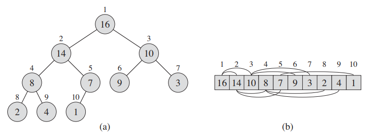
The (a) binary tree is represented using the (b) contiguous array ³. The number above each node is the index of that node in the array. We can observe that the indexes are increasing from top to bottom from left to right. The number inside each node is the key, or the value of the node. Given a node at index , we can easily compute its parent, left and right child:

def left(i):
    return 2 * i

def right(i):
    return left(i) + 1

def parent(i):
    return math.floor(i/2)

Heapify

To maintain the max heap property, the heapify algorithm is applied. Heapify receives a heap and an index to a subtree, which will be ordered by comparing and swapping the values of its child nodes. Heapify checks if the root node of the subtree is lesser than its childs. If it is, the nodes are swapped. This operation is also known as sift down.

If there is a swap, heapify executes again at the subtree of the node that was swapped. This is needed because the subtree might not be a heap due to the swap. This can happen when the value of the node is smaller than its children. We can observe this behavior in this animation made by CodesDope which ilustrates heapify ⁴:

def max_heapify(heap, i: int, m: int):
    l = left(i)
    r = right(i)
    max_value = i

    if l < m and heap[l] > heap[max_value]:
        max_value = l

    if r < m and heap[r] > heap[max_value]:
        max_value = r

    if max_value != i:
        swap(heap, i, max_value)
        max_heapify(heap, max_value, m)

Heapify runs in time, where is the height of the node which can be calculated by applying on the index of the node.

To build the heap, is applied to all nodes, starting from bottom nodes and moves towards the root node. It starts from the bottom because the subtrees of a node should already be heaps. The nodes at the bottom can be indexed by using when the heap is implemented using a contiguos array.

def build_heap(heap):
    heap_size = len(heap)
    n = math.floor(heap_size/2)

    for i in range(n+1):
        max_heapify(heap, n - i, heap_size)

Heap sorting

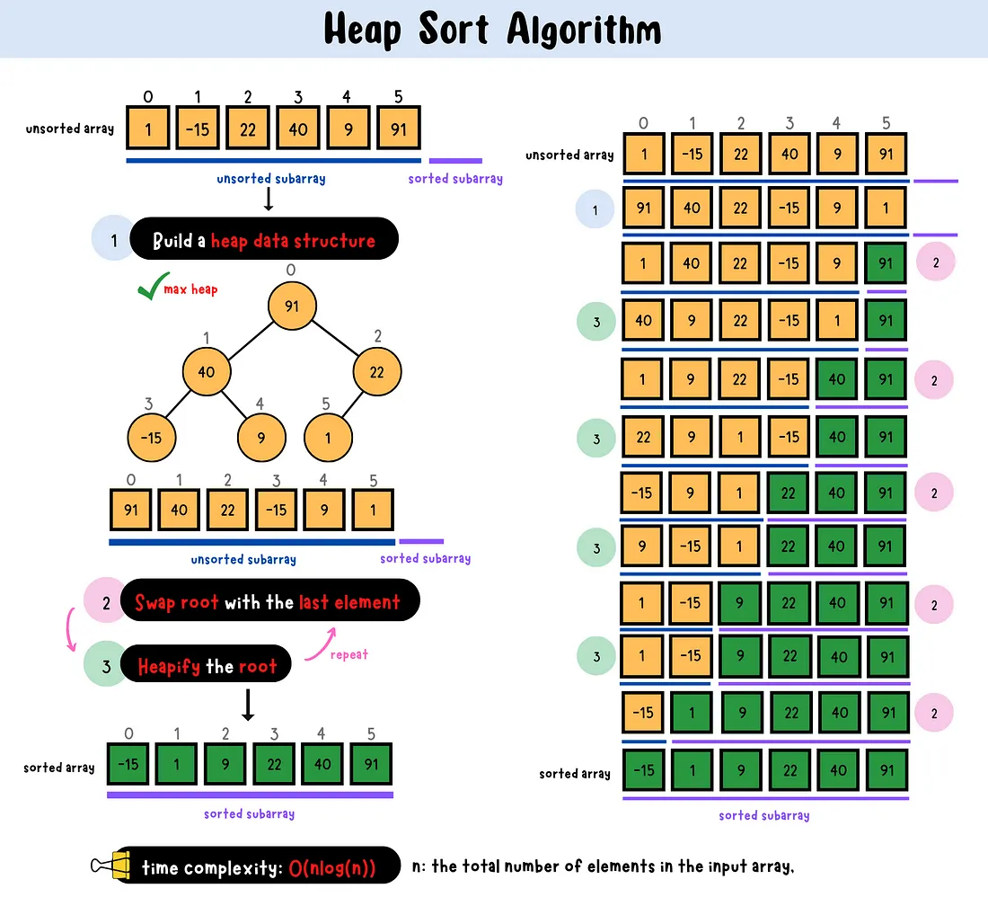
Intuitively, the heapsort algorithm builds the heap using and iteractively swaps the position of the root node, which is the largest element in the heap, with the lowest leaf node. Then is applied to maintain the max heap property, but without considering the last node which was sorted. This process continues until the last element in the heap is sorted.

def heapsort(heap):
    build_heap(heap)
    heap_size = len(heap)

    for i in range(heap_size):
        n = heap_size - 1 - i
        swap(heap, 0, n)
        max_heapify(heap, 0, n)

This is an ilustrated animation of the algorithm made by CodesDope ⁴.

Because , which runs in time, is applied times, the time complexity of heapsort is which is the best time complexity for sorting algorithms that use comparisons.

Stability

Heapsort is not a stable sorting algorithm due to the procedure which is executed in every iteration. Nodes with the same keys can change their relative position. This can happen because the lowest node is swapped with the root node, and during the node is moved to the bottomost subtree which might differ from node’s initial position. To illustrate this behavior, consider the following heap:

heap = [
   (4, "Alice"),
   (6, "Mart"),
   (6, "Kage"),
   (3, "Bob"),
   (3, "John"),
   (5, "Robert"),
   (1, "Plato"),
]

When sorted using heapsort it outputs:

heapsort(heap)

# [
#  1: Plato,
#  3: John, 
#  3: Bob, 
#  4: Alice, 
#  5: Robert, 
#  6: Kage, 
#  6: Mart
# ]

We can observe that the relative position of Mart and Kage as well as Bob and John are swapped. This reveals that heapsort is indeed not stable.

Conclusion

We explored heapsort an efficient, both in time and space complexity, sorting algorithm which uses the heap data structure. Due to the left-complete property, we learned that it is possible to use a contiguos array to represent a binary tree, which allows heapsort to maintain a constant space complexity of .

We explored the properties of the left-complete binary tree and how operation contributes to heapsort’s time complexity of . We also demonstrated the unstability of heapsort, which is an important property of the sorting algorithms, which can be relevant depending on the use case.

I hope you have enjoyed the explanations, have a wonderful day.